Data Set Development
Data Aquisition and Processing
Determining time of year when rivers are at mean discharge
NARWidth is composed of planform morphometric measurements of rivers at approximately mean discharge. Temporal fluctuations in discharge are a combined result of unpredictable events (e.g. storms and droughts) and more predictable seasonal variability in runoff. Unfortunately, no high-density, global-scale, daily discharge data sets exist to track the specific days that rivers are at their mean discharge. We approached the problem by determining the time of year that rivers in different parts of the globe are most likely to be at mean discharge.
To determine the optimal time of year to measure rivers, we used an international archive of long-term (>10 years) mean monthly discharge measurements from the Global Runoff Data Centre(GRDC)[GRDC, 2011] composed of 1920 gauges in North America. For each station with a complete record (i.e. no missing data values), we constructed a mean monthly hydrograph and calculated the mean and standard deviation (1σ) for all monthly measurements (Figure 1a). All months with discharges that fall within one standard deviation of the mean were scored according the following equation,
score(m) = Qμ - 0.5*Qm - 0.25*(Qm-1 + Qm+1),
where m is a given month being scored, Qμ is the mean of all monthly discharges, Qm is the mean monthly discharge of the given month, Qm-1 is the mean monthly discharge one month before month m, and Qm+1 is the mean monthly discharge of the month after month m. River discharge is more likely to be at or near the overall mean value during months with lower scores. Thus at each gauge station we produced a list of months that were ranked by the probability that the river was at mean discharge. To assign the monthly rankings from the gauge stations to each Landsat tile (landsat.usgs.gov), we considered both the proximity to gauge location and the monthly ranking. For example, the highest ranked month from the nearest gauge station has the greatest weight in setting the monthly preference order at a given Landsat tile. Each Landsat footprint is assigned at least one monthly preference and up to five ordered preferences (Figure 1b).
Figure 1. Method for determining the time of year to analyze rivers. a) Example mean monthly hydrograph (George River, CN). Months with discharges within one standard deviation (gray box) of the mean discharge (dashed horizontal line) are ranked (blue numbers) based on their discharge and that of their two neighboring months (equation 1). The best month to measure river width is September. b) Month that rivers are most likely to be at mean discharge for each Landsat tile.
Landsat Imagery Acquisition
Landsat TM and ETM+ (SLC-on) scenes were acquired from two data sources. We automatically downloaded the majority of scenes (1071 out of a total of 1756 scenes) from the Global Land Cover Facility (GLCF). The highest ranking scene was downloaded first. Upon download, each scene was visually inspected for flaws (e.g. clouds, river ice, shadows, flooding, no rivers) and either kept for use or discarded. If discarded, the next highest ranking scene was automatically downloaded. Once all available imagery was downloaded from the GLCF site, we manually downloaded Landsat scenes from the (USGS) in order of monthly preference. Thirty-four Landsat tiles in North America, located primarily in the tropics, had no cloud-free scenes available. To address this problem, we developed a program in IDL (version 8.0) that identified clouds based on their spectral signature and splices two or more complementary scenes together to eliminate clouds [Martinuzzi et al., 2007]. Fourteen Landsat tiles located high in the Canadian Archipelago had no scenes free of cloud and ice available during any of the monthly preferences listed. These scenes most likely have few if any wide rivers because they are located on relatively small and glacially dominated islands. Apart from these fourteen tiles, we successfully acquired imagery for all observable rivers in North America.
Image Processing
To classify water, we used the modified normalized difference water index,
MNDWI = (green-MIR)/(green+MIR),
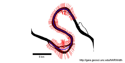
where MIR is the middle infrared band (e.g. TM Band 5) and green is the green band (i.e. TM Band 2) [Xu, 2006]. We applied the MNDWI formula to all Landsat scenes, mosaicked, and clipped images to 4° Latitude by 6° Longitude tiles. We then created a binary water mask by applying a dynamic threshold [Li and Sheng, 2012] which was visually inspected and corrected for any gaps in continuity and classification errors. These errors stem from sources including river view obstruction by topographic shadows, bridges, or dams, or the erroneous inclusion of swamps, large lakes, or deltas in the river network. RivWidth (version 0.4) calculated a channel centerline for all river reaches longer than 10 km (Figure 2). After RivWidth runs on a mosaic image, we visually inspected the RivWidth output for errors.
Figure 2. The RivWidth program calculates a river centerline (blue) from a binary river mask (black) derived from Landsat imagery [modified from Miller et al., 2014]. At each centerline pixel, RivWidth computes the river width and braiding index. A river length was computed at each width measurement by calculating the Euclidean distance between each centerline pixel and the next adjacent centerline pixel.
Reservoir and Lake Classification
Reservoirs and lakes connected to the fluvial network were labeled using GIS methods and several water body data sets: 1) the Global Lakes and Wet Lands Database (GLWD) [Lehner and Doll, 2004]; 2) the Global Reservoir and Dam Database (GRanD) [Lehner et al., 2011]; 3) the U.S. and Canada Water Polygons data set [TomTom North America, 2012]; and 4) the Mexico Water Bodies data set [Sistemas de Informacion Geografica, 2008]. The locations of lakes and reservoirs were then visually inspected and corrected in ArcGIS.
Validation
NARWidth Validation Methods
NARWidth width measurements were validated using 1,049 stream flow and river width records from the USGS and the Water Survey of Canada (WSC). At each gauge location, we estimated the river width at mean annual discharge and compared this value to the average of the five spatially closest RivWidth measurements (Figure 3). We excluded river width measurements that: 1) were taken more than 200 m upstream or downstream from the gauge station; 2) were taken when river ice was observed; or 3) were labelled as “Poor” measurements. We then took the mean of all width measurements that were taken when river discharge was within 5% of the mean annual discharge (red dots, Figure 3) and compared mean in situ width with the mean width of the five nearest NARWidth river width measurements.
Figure 3. Example in situ river discharge-width rating curve used to validate NARWidth. Mean annual discharge was calculated using daily discharge over at least a 10 year period (black line). The corresponding river width (red line) was then compared to the mean of the five nearest Landsat-derived NARWidth measurements at that location (blue line).
NARWidth Validation
NARWidth width measurements show very little mean bias (-0.35 m) relative to in situ width measurements at mean discharge, suggesting the Landsat scenes were sampled at times that, on average, matched mean discharge timing. The RMSE between NARWidth and in situ widths is 38.0 m, a length similar to the minimum theoretical uncertainty of Landsat-derived river widths calculated from a binary water mask [Pavelsky and Smith, 2008]. The RMSE value also incorporates several other sources of error, including differences in discharge between the remotely sensed and in situ measurements and error in the in situ width measurements.
To avoid bias from outliers, we used the Theil-Sen median estimator [Sen, 1968] to derive a robust linear regression between NARWidth and in situ width measurements (Figure 4). Regression of in situ widths >=100 m yields a slope that deviates by 3% from unity, but inclusion of all river width data (>=30 m) produces a slope that deviates by 16%. This deviation is expected because NARWidth is more likely to include overestimates of river width compared to underestimates where river width approaches the resolution of the Landsat imagery. For example, NARWidth never includes underestimates of 30 m wide rivers because they are narrower than one Landsat pixel, but it will include overestimates of these rivers. Goodness of fit (rs = 0.83) was characterized using Spearman’s nonparametric correlation coefficient [Spearman, 1904]. Overall, comparison with in situ measurements suggests that NARWidth provides, on average, an accurate representation of river widths at mean annual discharge to the extent that this is possible from Landsat imagery.
Figure 4. NARWidth river width validation. NARWidth widths were compared to USGS and WSC in situ river width measurements at 1,049 locations.
References
GRDC (2011), Long-Term Mean Monthly Discharges and Annual Characteristics of GRDC Station, edited by G. R. D. Centre, Federal Institute of Hydrology (BfG), Koblenz, Germany.
Lehner, B., and P. Doll (2004), Development and validation of a global database of lakes, reservoirs and wetlands, J. Hydrol., 296(1-4), 1-22, doi: 10.1016/j.jhydrol.2004.03.028.
Lehner, B., et al. (2011), Global Reservoir and Dam Database, Version 1 (GRanDv1): Reservoirs, Revision 01, edited, Global Water System Project (GWSP).
Li, J., and Y. Sheng (2012), An automated scheme for glacial lake dynamics mapping using Landsat imagery and digital elevation models: a case study in the Himalayas, Int. J. Remote Sens., 33(16), 5194-5213, doi: 10.1080/01431161.2012.657370.
Martinuzzi, S. n., W. A. Gould, and O. M. Ramos Gonzalez (2007), Creating cloud-free Landsat ETM+ data sets in tropical landscapes cloud and cloud-shadow removal, U.S. Dept. of Agriculture, Forest Service, International Institute of Tropical Forestry, Rio Piedras, PR.
Miller, Z. F., T. M. Pavelsky, and G. H. Allen (2014), Quantifying river form variations in the Mississippi Basin using remotely sensed imagery, Hydrol. Earth Syst. Sci., 18(12), 4883-4895, doi: 10.5194/hess-18-4883-2014.
Pavelsky, T. M., and L. C. Smith (2008), RivWidth: A Software Tool for the Calculation of River Widths From Remotely Sensed Imagery, Geoscience and Remote Sensing Letters, IEEE, 5(1), 70-73, doi: 10.1109/lgrs.2007.908305.
Sen, P. K. (1968), Estimates of the Regression Coefficient Based on Kendall's Tau, J. Am. Stat. Assoc., 63(324), 1379-1389, doi: 10.1080/01621459.1968.10480934.
Sistemas de Informacion Geografica, S. A. (2008), Mexico Water Bodies [electronic resource], edited, Esri, Redlands, California, USA.
Spearman, C. (1904), The Proof and Measurement of Association between Two Things, Am. J. Psychol., 15(1), 72-101, doi: 10.2307/1412159.
TomTom North America, I. (2012), U.S. and Canada Water Polygons [electronic resource], edited, Esri, Redlands, California, USA.
Xu, H. (2006), Modification of normalised difference water index (NDWI) to enhance open water features in remotely sensed imagery, Int. J. Remote Sens., 27(14), 3025-3033, doi: 10.1080/01431160600589179.


